Bucky's MySQL Tutorials

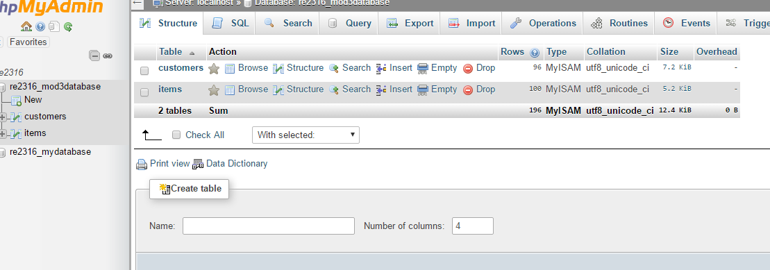
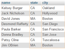
Bucky's MySQL tutorials give an introduction to creating a database and the various of ways of working with it. Videos 1-3 give a brief introduction to databases and explain how to get a server on which to operate a database, and culminate in creating a database of your own. Using the sample data Bucky provided, I created a database and filled it with information, as seen in the image below.

Part 4 demonstrates the SHOW and SELECT statements. The SHOW command could show all of the databases on the server or tables in the database, and the SELECT command would display specific information from tables. For example, the SELECT city FROM customers would show all of the cities from the customers table.

Part 5 continues with SQL commands, demonstrating running multiple queries at the same time and emphasizing that each statement must be ended with a semicolon. It also enforces that SQL commands are typically written in all caps - while it isn't a requirement for the statements to run, it is an important standard for readability purposes.

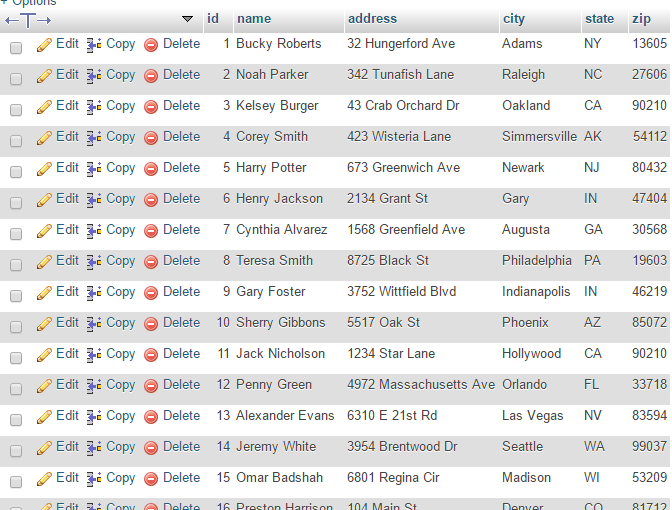
Part 6 expands on the SELECT statement, demonstrating getting multiple columns with one SELECT statement. For example, the command SELECT name, zip FROM customers will display the columns name and zip together. It almost introduces the wildcard (*) character, which will display ALL columns in the table. The following output is displayed when using the command SELECT * FROM customer:

Part 7 introduces the DISTINCT and LIMIT keywords - DISTINCT will eliminate all duplicate results from a query, and LIMIT will specify the number of results. For example, the statement SELECT id, name FROM customers LIMIT 5, 10 will begin at item 5, and display 10 entries.

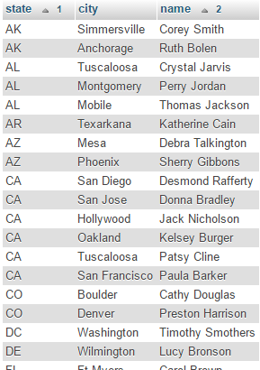
Part 8 describes fully qualified names, which give both the table name and column in one name. For example, customers.address is a fully qualified name. More importantly in this lesson, Bucky introduces sorting. The ORDER BY statement will arrange results alphabetically A-Z by default. The ORDER BY statement can be specified to order in exact ways; for example, the statement SELECT state, city, name FROM customers ORDER BY state, name will take the first criteria, state, and order by that - and within those states, the entries are ordered by name alphabetically. You can see an example of this below.

Part 9 helps refine sorting, and allows you to sort in different directions. By default, MySQL will sort in ascending order, but the keyword DESC can be used to sort in descending order.

Part 10 allows the user to begin filtering data. The WHERE clause can be given a condition in order to give specific results; for example, the statement SELECT id, name FROM customers WHERE id=54 will only show the entry that has an ID number equal to 54. Different conditions can be utilized, such as != (not equal to), > (greater than), <= (less than or equal to), etc. The keyword BETWEEN can also be used to find entries that are between two parameters, such as BETWEEN 25 AND 30.

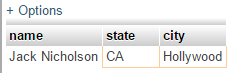
Part 11 expands on filtering using the AND and OR keywords. The AND statement will only return results for which all set parameters are true, where as the OR keyword will return results for which any of the parameters are true. The following images demonstrate this: the first set of results has been queried using an AND statement: SELECT name, state, city FROM customers WHERE state='CA' AND city='Hollywood'. The second image shows results that were queried using an OR statement: SELECT name, state, city FROM customers WHERE city='Boston' OR state='CA'.

Part 12 introduces the IN statement which allows for easier searching within mutliple parameters without having to use numerous OR statements. For example, SELECT name, state FROM customers WHERE state IN ('CA', 'NC', 'NY') will search for entries within that list of states. Conversely, the NOT IN statement can be used to search only for entries that do not contain these parameters.

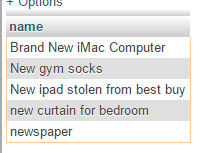
Part 13 introduces different search terms using the keyword LIKE and the % sign. The statement SELECT name FROM items WHERE name LIKE 'new%' will return all results who have names starting with the word 'new', and the % wildcard designates that it can be followed with any other characters or words. The % wildcard can be used before or after the search term to open the results in different directions. A demonstration of the query SELECT name FROM items WHERE name LIKE '%new%' is shown below.

Part 14 expands on the concept of wildcards, introducing the underscore. The underscore character searches for only a single character before the search term. For example, the query "_ boxes of frogs" would return 3 boxes of frogs and 7 boxes of frogs, but not 48 boxes of frogs.

Part 15 describes regular expressions, REGEXP, which allow for search of more complex patterns. The pipeline symbol (|) can be used as meaning "or"; for example, the query SELECT name FROM items WHERE name REGEXP 'gold|car' will search for items containing the word gold or car. A set can search for multiple items; for example, the query SELECT name FROM items WHERE name REGEXP '[1-5] boxes of frogs' will search for 1, 2, 3, 4, or 5 boxes of frogs. The negate symbol (^) can be used to inverse this search, and find anything BUT 1, 2, 3, 4, or 5 boxes of frogs.

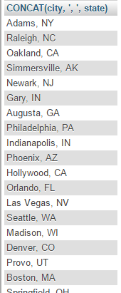
Part 16 delves into creating custom columns. You can use the keyword CONCAT, short for concatenate, to combine columns together and add characters. The following image demonstrates results generated by the statement SELECT CONCAT(city, ', ', state) FROM customers. A name, like new_address, can be assigned to this custom column by using the statement AS new_address after the CONCAT().

Part 17 introduces the concept of functions, which was touched upon briefly in the previous lesson which CONCAT(). Other examples of functions are UPPER(), which changes all letters to uppercase, SQRT(), which gives the square root of columns with numeric values, and aggregate functions such as AVG() and SUM(), which will average and sum, respectively, the values of all items in a column.

Part 18 continues to expand on aggregate functions, such as running these functions into custom columns.

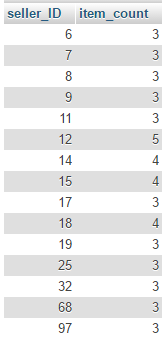
Part 19 introduces the statement GROUP BY, which allows you to display something like the number of items each seller is selling without having to run each query individually. The image below demonstrates this with the statement SELECT seller_ID, COUNT(*) AS item_count FROM items GROUP BY seller_id HAVING COUNT(*)>=3, and shows each seller that is selling 3 or more items.

Parts 20 and 21 describe subqueries, which will allow you to execute queries within queries. For example, you can find the average cost of items and then find only items that are greater than the average cost.

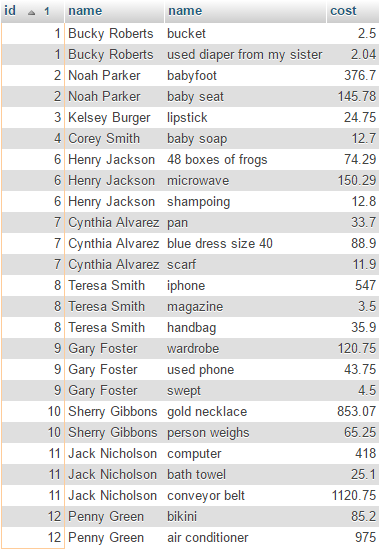
Part 22 discusses how to join tables, which is useful for avoiding repetitive information in an SQL query. This can be achieved using statement like SELECT customers.id, customers.name, items.name, items.cost FROM customers, items WHERE customers.id=seller_id ORDER BY customers.id, which will show the customers' names next to the ID number they match to. The following image is a demonstration of this statement:

Part 23 covers outer joins, and demonstrates how to nickname tables using the AS keyword. An outer join will display fields that do not have any fields associated with them as 'null'. For example, the following image is a demonstration of the outer join statement, SELECT customers.name, items.name FROM customers LEFT OUTER JOIN items ON customers.id=seller_id:

Part 24 introduces the UNION keyword, which will run two queries, but generate one set of data. While it's possible to achieve the same effect with WHERE clauses, UNION makes it simpler to read. The columns must be the same in order to use a UNION.

Part 25 explains full-text searching, which allows search within tables and displays and ranks results depending on relevancy. This type of search is also much faster than using regular expressions or the LIKE statement. You can use the term IN BOOLEAN MODE to specify the search by adding symbols like + (make sure this term is included) or - (make sure this term is not included). An example of this syntax is SELECT name, cost FROM items WHERE Match(name) Against('+baby -coat' IN BOOLEAN MODE).

Part 26 begins to edit databases, and in this part the INSERT INTO statement is introduced. A statement like INSERT INTO items(id,name,cost,seller_id,bids) VALUES('102', 'fish n chips', '7.99', '1', '0') will add each item in quotation marks into their respective columns.

Part 27 expands on this and allows adding of multiple rows. Instead of typing numerous INSERT INTO statements, one can be used and each row can be separated by commas. For example, the statements INSERT INTO items(id, name, cost, seller_id, bids) VALUES('104', 'beef chops', '7.99', '1', '0'), ('105', 'jelly pockets', '4.50', '1', '0'), ('106', 'sack of ham', '9.95', '1', '0') will insert three rows with this information.

Part 28 allows further editing of the database using the UPDATE and DELETE keywords. For example, UPDATE items SET name='frog paste', bids=66 WHERE id=106 will update the name and bids of the item ONLY with ID 106 instead of editing the names of the entire column. If you wanted to delete the information on this row, the statement DELETE FROM items WHERE id=106 will do so.

Part 29 demonstrates how to make a table through the command line in MySQL, and part 30 allows customization of the columns added such as not allowing null values (NOT NULL) for a field or automatically incrementing a primary key value with AUTO_INCREMENT.

Table manipulation continues in part 31, and with the ALTER TABLE statement extra columns can be added and DROP COLUMN can get rid of a column. The table can also be renamed. The final sections of this series, part 32 and 33, show how to view items in the database in different ways and save these views, which dynamically update, for easy viewing later.